Tharammal: Influence of Last Glacial Maximum boundary conditions on the global water isotope distribution in an atmospheric general circulation model

Fig. 3. Annual mean difference of surface temperature (C) of (a) GHG, (b) albedo, (c) topography, (d) orbital, (e) SST, and (f) LGM combined experiments from the control run. Anomalies in the surface temperature at the margins of the Ross and Weddell seas in the SST and the LGM-combined experiments are stippled because the respective grid cells were erroneously defined as ocean.
Influence of Last Glacial Maximum boundary conditions on the global water isotope distribution in an atmospheric general circulation model

Abstract. To understand the validity of d 18 O proxy records as indicators of past temperature change, a series of experiments was conducted using an atmospheric general circulation model fitted with water isotope tracers (Community Atmosphere Model version 3.0, IsoCAM). A pre-industrial simulation was performed as the control experiment, as well as a simulation with all the boundary conditions set to Last Glacial Maximum (LGM) values. Results from the pre-industrial and LGM simulations were compared to experiments in which the influence of individual boundary conditions (greenhouse gases, ice sheet albedo and topography, sea surface temperature (SST), and orbital parameters) were changed each at a time to assess their individual impact. The experiments were designed in order to analyze the spatial variations of the oxygen isotopic composition of precipitation (d 18 O precip ) in response to individual climate factors. The change in topography (due to the change in land ice cover) played a significant role in reducing the surface temperature and d 18 O precip over North America. Exposed shelf areas and the ice sheet albedo reduced the Northern Hemisphere surface temperature and d 18 O precip further. A global mean cooling of 4.1 °C was simulated with combined LGM boundary conditions compared to the control simulation, which was in agreement with previous experiments using the fully coupled Community Climate System Model (CCSM3). Large reductions in d 18 O precip over the LGM ice sheets were strongly linked to the temperature decrease over them. The SST and ice sheet topography changes were responsible for most of the changes in the climate and hence the d 18 O precip distribution among the simulations.

Influence of Last Glacial Maximum boundary conditions on the global water isotope distribution in an atmospheric general circulation model
T. Tharammal, A. Paul, U. Merkel, and D. Noone
Clim. Past, 9, 789-809, 2013
http://www.clim-past.net/9/789/2013/
doi:10.5194/cp-9-789-2013
© Author(s) 2013. This work is distributed
under the Creative Commons Attribution 3.0 License.

Willet: HadISDH: an updateable land surface specific humidity product for climate monitoring

Fig. 13. Comparison of large-scale annual average time series from HadISDH land specific humidity with land surface air temperature from CRUTEM4 (Jones et al., 2012) and sea surface temperature from HadSST3 (Kennedy et al., 2011a, b), including uncertainty ranges. Temperature data have been adjusted to have a zero mean over the 1976–2005 climatology period of HadISDH. Correlations between the land air temperature and SST and land surface humidity have been performed on the detrended time series.
HadISDH: an updateable land surface specific humidity product for climate monitoring

HadISDH is a near-global land surface specific humidity monitoring product providing monthly means from 1973 onwards over large-scale grids. Presentedherein to 2012, annual updates are anticipated. HadISDH is an update to the land component of HadCRUH, utilising the global high-resolution land surface station product HadISD as a basis. HadISD, in turn, uses an updated versionof NOAA’s Integrated Surface Database. Intensive automated quality control has been undertaken at the individual observation level, as part of HadISD processing. The data have been subsequently run through the pairwise homogenisation algorithm developed for NCDC’s US Historical Climatology Network monthly temperature product. For the first time, uncertainty estimates are provided at the grid-box spatial scale and monthly timescale.

HadISDH: an updateable land surface specific humidity product for climate monitoring
K. M. Willett, C. N. Williams Jr., R. J. H. Dunn, P. W. Thorne, S. Bell, M. de Podesta, P. D. Jones, and D. E. Parker
Clim. Past, 9, 657-677, 2013
http://www.clim-past.net/9/657/2013/
doi:10.5194/cp-9-657-2013
© Author(s) 2013. This work is distributed
under the Creative Commons Attribution 3.0 License.

Fig. 9. Decadal trends in specific humidity for HadCRUH versus HadISDH over the 1973–2003 period of record. Trends have been estimated using the median of pairwise slopes (Sen, 1968; Lanzante, 1996) method. Where intervals defined by the 95% confidence limits on the median of the slopes are both of the same sign as the median trend presented in the grid boxes, the trend is presumed to be significantly different from a zero trend. This is indicated by a black dot within the grid box. This means that there is higher confidence in the direction of the trend, but not necessarily the magnitude. The spread of the confidence interval provides the confidence in the magnitude; these values are available online at http://www.metoffice.gov.uk/hadobs/hadisdh. Note non-linear colour bars.

Fig. 11. Decadal trends in specific humidity for HadISDH over 1973–2012. Trends are fitted and confidence assigned as described in Fig. 9. Note non-linear colour bars.

Winnick: Stable isotopic evidence of El Niño-like atmospheric circulation in the Pliocene western United States

Fig. 1. Modern El Ni˜no precipitation anomalies, isotope localities, and reconstructed Pliocene conditions. Anomalous annual El Ni˜no precipitation calculated with CMAP precipitation data from 1979– 2008; CMAP precipitation data provided by the NOAA/OAR/ESRL PSD, Boulder, CO, USA, from their Web site at http://www.esrl. noaa.gov/psd/. Purple stars show isotope record localities used in this study. Blue circles represent reconstructions of wetter-thanmodern Pliocene conditions, and red circles represent reconstructions of drier-than-modern Pliocene conditions.
Stable isotopic evidence of El Niño-like atmospheric circulation in the Pliocene western United States

Abstract. Understanding how the hydrologic cycle has responded to warmer global temperatures in the past is especially important today as concentrations of CO 2 in the atmosphere continue to increase due to human activities. The Pliocene offers an ideal window into a climate system that has equilibrated with current atmospheric p CO 2 . During the Pliocene the western United States was wetter than modern, an observation at odds with our current understanding of future warming scenarios, which involve the expansion and poleward migration of the subtropical dry zone. Here we compare Pliocene oxygen isotope profiles of pedogenic carbonates across the western US to modern isotopic anomalies in precipitation between phases of the El Niño-Southern Oscillation (ENSO). We find that when accounting for seasonality of carbonate formation, isotopic changes through the late Pliocene match modern precipitation isotopic anomalies in El Niño years. Furthermore, isotopic shifts through the late Pliocene mirror changes through the early Pleistocene, which likely represents the southward migration of the westerly storm track caused by growth of the Laurentide ice sheet. We propose that the westerly storm track migrated northward through the late Pliocene with the development of the modern cold tongue in the east equatorial Pacific, then returned southward with widespread glaciation in the Northern Hemisphere – a scenario supported by terrestrial climate proxies across the US. Together these data support the proposed existence of background El Niño-like conditions in western North America during the warm Pliocene. If the earth behaves similarly with future warming, this observation has important implications with regard to the amount and distribution of precipitation in western North America.

Stable isotopic evidence of El Niño-like atmospheric circulation in the Pliocene western United States
M. J. Winnick, J. M. Welker, and C. P. Chamberlain
Clim. Past, 9, 903-912, 2013
http://www.clim-past.net/9/903/2013/
doi:10.5194/cp-9-903-2013
© Author(s) 2013. This work is distributed
under the Creative Commons Attribution 3.0 License.

Morrill: Model sensitivity to North Atlantic freshwater forcing at 8.2 ka

Fig. 3. Time series of AMOC intensity anomalies following the MWP, expressed as a fraction of the long-term control mean. The MWP of 2.5 Sv for one year was added at Model year 1. AMOC intensity is defined as the maximum value of the overturning streamfunction below 500 m water depth (excludes shallow wind-driven overturning). Heavy lines are decadal averages. Vertical lines on the right show the 2-sigma range of interannual variability in the control simulations, and are not shown for ModelE-R since only 30 yr control averages are available.

Model sensitivity to North Atlantic freshwater forcing at 8.2 ka

We compared four simulations of the 8.2 ka event to assess climate modelsensitivity and skill in responding to North Atlantic freshwaterperturbations. All of the simulations used the same freshwater forcing, 2.5 Sv for one year, applied to either the Hudson Bay(northeastern Canada) or Labrador Sea (between Canada’s Labrador coast and Greenland). Thisfreshwater pulse induced a decadal-mean slowdown of 10–25% in theAtlantic Meridional Overturning Circulation (AMOC) of the models and causeda large-scale pattern of climate anomalies that matched proxy evidence forcooling in the Northern Hemisphere and a southward shift of theIntertropical Convergence Zone. The multi-model ensemble generatedtemperature anomalies that were just half as large as those fromquantitative proxy reconstructions, however. Also, the duration of AMOC andclimate anomalies in three of the simulations was only several decades,significantly shorter than the duration of ~150 yr in thepaleoclimate record. Possible reasons for these discrepancies includeincorrect representation of the early Holocene climate and ocean state inthe North Atlantic and uncertainties in the freshwater forcing estimates.

Model sensitivity to North Atlantic freshwater forcing at 8.2 ka
C. Morrill, A. N. LeGrande, H. Renssen, P. Bakker, and B. L. Otto-Bliesner
Clim. Past, 9, 955-968, 2013
http://www.clim-past.net/9/955/2013/
doi:10.5194/cp-9-955-2013
© Author(s) 2013. This work is distributed
under the Creative Commons Attribution 3.0 License.

Kavvada: AMO’s structure and climate footprint in observations and IPCC AR5 climate simulations

All-season regressions of standardized smoothed AMO indices on SSTs for the winter 1900–fall 1999 period. Regressions for the models are calculated for each ensemble member separately and then an average is computed for each model. Red/blue shading denotes positive/negative SST anomalies; contour interval is 0.1 K. The indices are constructed by first calculating a spatial average of SST anomalies over the (5°–75°W, 0°–60°N) region and then detrended, using the least squares method. The indices are finally smoothed by applying a 1-2-1 binomial filter 50 times and normalized by using their standard deviation. Regressions are shown after 5 applications of smth9 in the GRADS plotting software. Bottom Panel Observed HadISST smoothed AMO index and other four model-derived smoothed AMO indices which have the highest correlations, R, with the observed index: GFDL-CM3, Ensemble 5 (R = 0.75), UKMO-HADCM3, Ensemble 4 (R = 0.56), ECHAM6/MPI-ESM-LR, Ensemble 3 (R = 0.01) and CCSM4 Ensemble 4 (R = 0.29). The correlation range for the different ensembles within each model is shown adjacent to the model’s name

ABSTRACT: This study aims to characterize the spatiotemporal features of the low frequency Atlantic Multidecadal Oscillation (AMO), its oceanic and atmospheric footprint and its associated hydroclimate impact. To accomplish this, we compare and evaluate the representation of AMO-related features both in observations and in historical simulations of the twentieth century climate from models participating in the IPCC’s CMIP5 project. Climate models from international leading research institutions are chosen: CCSM4, GFDL-CM3, UKMO-HadCM3 and ECHAM6/MPI-ESM-LR. Each model employed includes at least three and as many as nine ensemble members. Our analysis suggests that the four models underestimate the characteristic period of the AMO, as well as its temporal variability; this is associated with an underestimation/overestimation of spectral peaks in the 70–80 year/10–20 year range. The four models manifest the mid-latitude focus of the AMO-related SST anomalies, as well as certain features of its subsurface heat content signal. However, they are limited when it comes to simulating some of the key oceanic and atmospheric footprints of the phenomenon, such as its signature on subsurface salinity, oceanic heat content and geopotential height anomalies. Thus, it is not surprising that the models are unable to capture the majority of the associated hydroclimate impact on the neighboring continents, including underestimation of the surface warming that is linked to the positive phase of the AMO and is critical for the models to be trusted on projections of future climate and decadal predictions.

AMO’s structure and climate footprint in observations and IPCC AR5 climate simulations
Argyro Kavvada, Alfredo Ruiz-Barradas and Sumant Nigam

Climate Dynamics
Observational, Theoretical and Computational Research on the Climate System
10.1007/s00382-013-1712-1

Argyro Kavvada
Email: argyrok@atmos.umd.edu
Received: 4 June 2012
Accepted: 20 February 2013
Published online: 7 March 2013

Holland and Bruyère: Recent intense hurricane response to global climate change

Fig 3. Anthropogenic influence on: a annual frequency of global tropical cyclones and hurricanes; b hurricane proportions in each of the Saffir–Simpson hurricane categories

Fig 4. Relationship of anthropogenic change defined from a CMIP3 and, b CCSM4 with annual proportions of Cat 1–2 and Cat 4–5 hurricanes. Note the different scales for the ACCI. A 5-year running mean smoother has been used (indicated by the SM in the legend), thin solid (dashed) lines indicate linear (quadratic) trends, and all variances have p 0.01 (using unsmoothed data)

ABSTRACT: An Anthropogenic Climate Change Index (ACCI) is developed and used to investigate the potential global warming contribution to current tropical cyclone activity. The ACCI is defined as the difference between the means of ensembles of climate simulations with and without anthropogenic gases and aerosols. This index indicates that the bulk of the current anthropogenic warming has occurred in the past four decades, which enables improved confidence in assessing hurricane changes as it removes many of the data issues from previous eras. We find no anthropogenic signal in annual global tropical cyclone or hurricane frequencies. But a strong signal is found in proportions of both weaker and stronger hurricanes: the proportion of Category 4 and 5 hurricanes has increased at a rate of ~25–30 % per °C of global warming after accounting for analysis and observing system changes. This has been balanced by a similar decrease in Category 1 and 2 hurricane proportions, leading to development of a distinctly bimodal intensity distribution, with the secondary maximum at Category 4 hurricanes. This global signal is reproduced in all ocean basins. The observed increase in Category 4–5 hurricanes may not continue at the same rate with future global warming. The analysis suggests that following an initial climate increase in intense hurricane proportions a saturation level will be reached beyond which any further global warming will have little effect.

Recent intense hurricane response to global climate change
Greg Holland and Cindy L. Bruyère

Climate Dynamics
Observational, Theoretical and Computational Research on the Climate System
http://dx.doi.org/10.1007/s00382-013-1713-0

Greg Holland
Received: 5 September 2012
Accepted: 21 February 2013
Published online: 15 March 2013

Read more …
Climate Attribution Alchemy (Pielke Jr)

Stolzea: Solar influence on climate variability and human development during the Neolithic: evidence from a high-resolution multi-proxy record from Templevanny Lough, County Sligo, Ireland

Fig. 9. Precipitation and temperature reconstruction from the Carrowkeel–Keshcorran area between 4000 and 2600 BC compared to variations in the production rate of the cosmogenic isotopes 14C and 10Be and periods of human development and archaeological presence in Ireland. Grey shading denotes periods of warmer and drier conditions inferred from the Carrowkeel–Keshcorran archives. References: (1) Muscheler et al. (2005); (2) Vonmoos et al. (2006); (3) references in Stolze et al. (2012); (4) Turney et al. (2006); (5) Sheridan (1995).

ABSTRACT: The relationship between climatic variations, vegetation dynamics and early human activity between c. 4150–2860 BC was reconstructed from a high-resolution pollen and geochemical record obtained from a small lake located in County Sligo, Ireland. The proxy record suggests the existence of a woodland with a largely closed canopy at the start of the fourth millennium BC. Only minor human disturbance is recorded. Following an episode of increased rainfall at c. 3990 BC, a decrease in the elm population occurred between c. 3970 and 3820 BC. This coincided with a period of warming and drying climatic conditions and an initial increase in anthropogenic activities. A second episode of high precipitation between c. 3830–3800 BC was followed by a steep increase in human impact on the landscape, which became most pronounced between c. 3740 and 3630 BC. At this time, the lake level of Templevanny Lough was at its lowest during the Neolithic.

The onset of wetter and cooler conditions after c. 3670 BC, representing the transition from the Early to the Middle Neolithic, coincided with a period of woodland recovery. The Middle Neolithic was characterised by pronounced climatic oscillations including periods of substantial rainfall between c. 3600 and 3500 BC and between c. 3500 and 3460 BC. A nearly century-long climatic amelioration between c. 3460–3370 BC facilitated a revival of human activity on a small scale around the lake. Abandonment of the area and full woodland recovery occurred after a period of particularly wet and cool conditions ranging from c. 3360–3290 BC. The pollen and geochemistry data suggest that the Late Neolithic was marked by a period of ameliorated conditions between c. 3110–3050 BC that was followed by two episodes of high rainfall at c. 3060–3030 BC and c. 2940–2900 BC.

The timing of the climatic shifts inferred from the Templevanny Lough record is in agreement with those of moisture/precipitation and temperature reconstructions from northern and western Europe and the Alps, suggesting that the studied period was characterised by a high-frequency climate variability. The results of the present study imply that human development during the Irish Neolithic was influenced by climatic variations. These climatic shifts correspond to variations in solar activity, suggesting a solar forcing on climate.

Solar influence on climate variability and human development during the Neolithic: evidence from a high-resolution multi-proxy record from Templevanny Lough, County Sligo, Ireland
Susann Stolzea, Raimund Muschelerb, Walter Dörflerc, Oliver Nellea
Quaternary Science Reviews
Volume 67, 1 May 2013, Pages 138–159
http://dx.doi.org/10.1016/j.quascirev.2013.01.013

Frame and Stone: Assessment of the first consensus prediction on climate change

The solid and dashed lines show the annual variations; the dotted lines show best-fit linear trends. Trend and annual variations are plotted as anomalies from the 1990 value of the trend fit.

ABSTRACT: In 1990, climate scientists from around the world wrote the First Assessment Report of the Intergovernmental Panel on Climate Change. It contained a prediction of the global mean temperature trend over the 1990–2030 period that, halfway through that period, seems accurate. This is all the more remarkable in hindsight, considering that a number of important external forcings were not included. So how did this success arise? In the end, the greenhouse-gas-induced warming is largely overwhelming the other forcings, which are only of secondary importance on the 20-year timescale.

Assessment of the first consensus prediction on climate change
David J. Frame & Dáithí A. Stone
Nature Climate Change 3, 357–359 (2013) doi:10.1038/nclimate1763
Received 31 July 2012 Accepted 01 November 2012 Published online 09 December 2012

TY – JOUR
AU – Frame, David J.
AU – Stone, Daithi A.
TI – Assessment of the first consensus prediction on climate change
JA – Nature Clim. Change
PY – 2013/04//print
VL – 3
IS – 4
SP – 357
EP – 359
PB – Nature Publishing Group
SN – 1758-678X
UR – http://dx.doi.org/10.1038/nclimate1763
M3 – 10.1038/nclimate1763
N1 – 10.1038/nclimate1763
ER –

Read more …
20-Year-Old Report Successfully Predicted Warming: Scientists (LiveScience)
Add Frame and Stone to the List of Papers Validating IPCC Warming Projections (Skeptical Science)
The IPCC was not right. Frame & Stone ignore main IPCC predictions (JoNova)

Guemas: Retrospective prediction of the global warming slowdown in the past decade

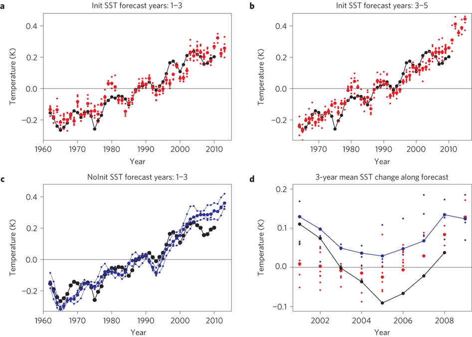
a–c, Global SST anomalies averaged between 60° S and 65° N and across forecast years 1–3 (a,c) and forecast years 3–5 (b). d, 3-year mean SST change along the forecasts. One large dot is shown for the ensemble mean of each forecast and small dots are shown for their members in Init (red). The equivalents in NoInit and in the observations are shown in blue and black respectively, joined by lines as they come from a continuous time series.

ABSTRACT: Despite a sustained production of anthropogenic greenhouse gases, the Earth’s mean near-surface temperature paused its rise during the 2000–2010 period1. To explain such a pause, an increase in ocean heat uptake below the superficial ocean layer2, 3 has been proposed to overcompensate for the Earth’s heat storage. Contributions have also been suggested from the deep prolonged solar minimum4, the stratospheric water vapour5, the stratospheric6 and tropospheric aerosols7. However, a robust attribution of this warming slowdown has not been achievable up to now. Here we show successful retrospective predictions of this warming slowdown up to 5 years ahead, the analysis of which allows us to attribute the onset of this slowdown to an increase in ocean heat uptake. Sensitivity experiments accounting only for the external radiative forcings do not reproduce the slowdown. The top-of-atmosphere net energy input remained in the [0.5–1] W m−2 interval during the past decade, which is successfully captured by our predictions. Most of this excess energy was absorbed in the top 700 m of the ocean at the onset of the warming pause, 65% of it in the tropical Pacific and Atlantic oceans. Our results hence point at the key role of the ocean heat uptake in the recent warming slowdown. The ability to predict retrospectively this slowdown not only strengthens our confidence in the robustness of our climate models, but also enhances the socio-economic relevance of operational decadal climate predictions.

Retrospective prediction of the global warming slowdown in the past decade
Virginie Guemas, Francisco J. Doblas-Reyes, Isabel Andreu-Burillo & Muhammad Asif
Nature Climate Change (2013) doi:10.1038/nclimate1863
Received 08 November 2012 Accepted 01 March 2013 Published online 07 April 2013

TY – JOUR
AU – Guemas, Virginie
AU – Doblas-Reyes, Francisco J.
AU – Andreu-Burillo, Isabel
AU – Asif, Muhammad
TI – Retrospective prediction of the global warming slowdown in the past decade
JA – Nature Clim. Change
PY – 2013/04/07/online
VL – advance online publication
SP –
EP –
PB – Nature Publishing Group
SN – 1758-6798
UR – http://dx.doi.org/10.1038/nclimate1863
L3 – 10.1038/nclimate1863
M3 – Letter
L3 – http://www.nature.com/nclimate/journal/vaop/ncurrent/abs/nclimate1863.html#supplementary-information
ER –

Read more …
Oceans May Explain Slowdown in Climate Change (Scientific Amercian)
New Study: When You Account For The Oceans, Global Warming Continues Apace (Climate Progress)
Guemas et al. Attribute Slowed Surface Warming to the Oceans (Skeptical Science)

Fire Weather: SE Australia

5.6 Fire weather

A substantial increase in fire weather risk is likely at most sites in south-eastern Australia. Such a risk may exist elsewhere in Australia, but this has yet to be examined.

Bushfires are an integral part of Australia’s environment. Its natural ecosystems have evolved with fire, and its landscapes and their biological diversity have been shaped by both historical and recent patterns of fire (Cary 2002). South-eastern Australia has the highest bushfire risk in spring, summer and autumn. This region has the reputation of being one of the three most fire-prone areas in the world, along with southern California and Mediterranean Europe.

Fire risk is influenced by a number of factors, including fuels, terrain, land management, fire suppression and weather. The Forest Fire Danger Index (FFDI) is used operationally to provide an indication of fire risk based on near-surface daily maximum temperature, daily total precipitation, 3 pm relative humidity and 3 pm wind speed. The FFDI has five intensity categories: low (less than 5), moderate (5-12), high (13-25), very high (25-49) and extreme (at least 50).

When the FFDI is extreme, a Total Fire Ban Day is usually declared. During the Canberra fires on 19 January 2003, the FFDI exceeded 100 (Figure 5.43).

Fire danger indices were calculated using daily weather records from 1974-2003 for 17 sites in south- eastern Australia (Hennessy et al. 2006). It was not possible to calculate changes in fire danger based on any of the CMIP3 models in Table 4.1. The results presented here are based on the study by Hennessy et al. (2006) using two climate change simulations with CSIRO’s Cubic Conformal Atmospheric Model (CCAM), which has 50 km resolution over Australia. One simulation (denoted CCAM Mark2) was driven by boundary conditions from the CSIRO Mark 2 coupled ocean-atmosphere model, while the other simulation (denoted CCAM Mark3) was driven by boundary conditions from the CSIRO Mark 3.0 model. Data from these simulations were then used to generate climate change scenarios per degree of global warming, including changes in daily weather variability. These changes were scaled by the IPCC (2001) global warming ranges for 2020 and 2050, then applied to the daily weather records from 1974-2003 at 17 sites in south-eastern Australia. Fire danger indices were then calculated for the modified 30 year datasets centred on 2020 and 2050 (Hennessy et al. 2006).

An increase in fire weather risk is simulated at most sites, including the average number of days when the FFDI rating is very high or extreme. The combined frequencies of days with very high and extreme FFDI ratings increase 4-25% by 2020 and 15-70% by 2050 (Table 5.7). For example, Canberra has an annual average of 25.6-28.6 very high or extreme fire danger days by 2020 and 27.9-38.3 days by 2050, compared with a present average of 23.1 days. The increase in fire weather risk is generally largest inland. Tasmania is relatively unaffected. It is likely that the higher fire weather risk in spring, summer and autumn will increasingly shift periods suitable for prescribed burning toward winter.

Climate Change in Australia – Technical Report 2007: Chapter 5.6

This study of CSIRO/CCAM results does predict increased fire risk in SE Australia, but does not appear to extend much of that risk to Tasmania.