Archive
Westcott and Jewsion: Weather Effects on Expected Corn and Soybean Yields

Corn Yield Model
A model for national corn yields was estimated over the past 25 years (1988-2012), thereby including both the 1988 and 2012 droughts. In addition to a trend variable, the model uses as explanatory variables mid-May planting progress, July weather (precipitation and average temperature), and a June precipitation shortfall measure in selected years. Including those variables helps explain previous yield variations and deviations from trend.Corn plantings by mid-May are important for yield potential because that allows more of the critical stages of crop development, particularly pollination, to occur earlier, before the most severe heat of the summer. Earlier pollination is also generally associated with less plant stress from moisture shortages. Most of the corn crop develops in July, so weather in that month is included in the model, including variables for both precipitation and temperature.
Finally, while weather in June is important for development of the corn crop (and June typically has lower temperatures and more rain than July), effects of June weather are typically small relative to July weather effects. However, extreme weather deviations from normal in June can have larger impacts, as seen in 2012 and in 1988. To represent that effect, the model uses a measure of the precipitation shortfall from average in years when June precipitation is in the lowest 10 percent tail of its statistical distribution. The mid-May planting progress variable is based on weekly data from USDA’s National Agricultural Statistics Service and is prorated to May 15 from adjacent weeks’ results for years that the statistic was not reported for that specific date. The weather data is from the National Oceanic and Atmospheric Administration.
The planting progress and weather data used is for eight key corn-producing States (Iowa, Illinois, Indiana, Ohio, Missouri, Minnesota, South Dakota, and Nebraska). Those eight States typically rank in the top 10 corn-producing States and accounted for an average of 76 percent of U.S. corn production over the estimation period. An aggregate measure for the eight States for each of those variables is constructed using harvested corn acres to weight State-specific observations.
The effects of mid-May planting progress and July temperatures on corn yield are each linear in the model—for those variables, each unit of change has a constant effect on yield. Similarly, the June precipitation shortfall variable is linear for the years it is nonzero. However, the effect of July precipitation is nonlinear in the model to reflect the asymmetric response of corn yields to different amounts of precipitation above and below its average. That is, reductions in corn yields when rainfall is below average are larger than gains in corn yields when rainfall is above average. The model uses a squared term for July precipitation to represent that asymmetric effect. The estimated regression equation (table 6) explains over 96 percent of the variation in national corn yields during the estimation period (more than 91 percent of the variation around the equation’s trend).
Weather Effects on Expected Corn and Soybean Yields
Paul C. Westcott, USDA, Economic Research Service
Michael Jewison, USDA, World Agricultural Outlook Board
The model assumes a linear trend for corn yields with a weather forced variation.

Note that as of June 12, 2013: U.S. corn production for 2013/14 was estimated 135 million bushels lower to 14.0 billion bushels. Corn yields for the upcoming year were projected at 156.5 bushels per acre, a 1.5 bushel decrease from May’s estimate. The decrease in yields is due to delays in planting in some of the highest producing corn states.
http://www.agweb.com/blog/Farmland_Forecast_148/
The baseline trend projection for 2013 is 163.6 bushels per acre, if this information from May is accurate: The 2013/14 corn yield is projected at 158.0 bushels per acre, 5.6 bushels below the weather adjusted trend presented at USDA’s Agricultural Outlook Forum in February [Edit: Confirmed here]
http://www.cattlenetwork.com/cattle-news/WASDE-Corn-yield-adjusted-lower–206929151.html
But even the new, lower projection is well above the 2011 and 2012 yields.
Lu: Cosmic-Ray-Driven Reaction and Greenhouse Effect of Halogenated Molecules: Culprits for Atmospheric Ozone Depletion and Global Climate Change

Abstract This study is focused on the effects of cosmic rays (solar activity) and halogenated molecules (mainly chlorofluorocarbons-CFCs) on atmospheric O3 depletion and global climate change. Brief reviews are first given on the cosmic-ray-driven electron-induced-reaction (CRE) theory for O3 depletion and the warming theory of CFCs for climate change. Then natural and anthropogenic contributions are examined in detail and separated well through in-depth statistical analyses of comprehensive measured datasets. For O3 loss, new statistical analyses of the CRE equation with observed data of total O3 and stratospheric temperature give high linear correlation coefficients >=0.92. After removal of the CR effect, a pronounced recovery by 20~25% of the Antarctic O3 hole is found, while no recovery of O3 loss in mid-latitudes has been observed. These results show both the dominance of the CRE mechanism and the success of the Montreal Protocol. For global climate change, in-depth analyses of observed data clearly show that the solar effect and human-made halogenated gases played the dominant role in Earth climate change prior to and after 1970, respectively. Remarkably, a statistical analysis gives a nearly zero correlation coefficient (R=-0.05) between global surface temperature and CO2 concentration in 1850-1970. In contrast, a nearly perfect linear correlation with R=0.96-0.97 is found between global surface temperature and total amount of stratospheric halogenated gases in 1970-2012. Further, a new theoretical calculation on the greenhouse effect of halogenated gases shows that they (mainly CFCs) could alone lead to the global surface temperature rise of ~0.6 deg C in 1970-2002. These results provide solid evidence that recent global warming was indeed caused by anthropogenic halogenated gases. Thus, a slow reversal of global temperature to the 1950 value is predicted for coming 5~7 decades.
Cosmic-Ray-Driven Reaction and Greenhouse Effect of Halogenated Molecules: Culprits for Atmospheric Ozone Depletion and Global Climate Change
Qing-Bin Lu
Comments: 24 pages, 12 figures; an updated version
Subjects: Atmospheric and Oceanic Physics (physics.ao-ph); Atomic and Molecular Clusters (physics.atm-clus); Chemical Physics (physics.chem-ph)
Journal reference: Int. J. Mod. Phys. B Vol. 27 (2013) 1350073 (38 pages)
DOI: 10.1142/S0217979213500732
Cite as: arXiv:1210.6844 [physics.ao-ph]
(or arXiv:1210.6844v2 [physics.ao-ph] for this version)
http://arxiv.org/abs/1210.6844
See also: Lu: from ‘interesting but incorrect’ to just wrong (Real Climate)
Dear Willard: Who needs words when one has letters and operators?
Peer-Reviewed Survey Finds Majority Of Scientists Skeptical Of Global Warming Crisis (Feb 2013)
http://www.forbes.com/sites/jamestaylor/2013/02/13/peer-reviewed-survey-finds-majority-of-scientists-skeptical-of-global-warming-crisis/
Regarding ad homininum (circumstantial)
Let X be AGW
1. Person A makes claim ~X.
2. Person B asserts that A makes claim ~X because it is in A’s interest to claim ~X.
3. Therefore claim ~X is false.
If Person B’s assetion is that ~X is false simply because the persons surveyed are petroleum engineers, I agree that argument is fallacious.
But there is a deeper problem. The author obscured the actual scope of the survey, so we aren’t even in agreement about the identity of “Person A”. And the identity of “Person A” has great relevance on the claim, since the whole op-ed is an argument from authority. In the beginning … “these skeptical scientists may indeed form a scientific consensus.” … and again in the end …”Now that we have access to hard surveys of scientists themselves” … much less the title of the piece … “Peer-Reviewed Survey Finds Majority Of Scientists Skeptical Of Global Warming Crisis”
How does the Forbes op-ed construct this consensus of scientists?
Through a fallacy of composition
1. A ‘consensus’ A makes the claim ~X OR ~Y
2. All A are an element of B
3. All B are an element of C
4. Therefore a ‘consensus’ of C makes the claim ~X OR ~Y
Where …
A is petroleum engineers from Alberta
B is geoscientists
C is scientists
X is ‘AGW’
Y is ‘crisis’
(note how Taylor mixes skepticism of causes (X) and consequences (Y) to construct his ‘majority’ and ‘consensus’)
The composition fallacy is more apparent when the actual group surveyed is revealed which is why it wasn’t and why noting the population surveyed isn’t fallacious. The source of the survey doesn’t prove/disprove ~X OR ~Y; it identifies the composition fallacy.
Selvam: Universal Inverse Power Law Distribution for Indian Region Rainfall
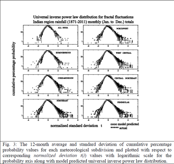
Space-time fluctuations of meteorological parameters exhibit selfsimilar fractal fluctuations. Fractal space-time fluctuations are generic to dynamical systems in nature such as fluid flows, spread of diseases, heart beat pattern, etc. A general systems theory developed by the author predicts universal inverse power law form incorporating the golden mean for the fractal fluctuations. The model predicted distribution is in close agreement with observed fractal fluctuations of all size scales in the monthly total Indian region rainfall for the 141 year period 1871 to 2011.
Universal Inverse Power Law Distribution for Indian Region Rainfall
From: A. Mary Selvam
[v1] Fri, 3 May 2013 09:52:00 GMT (434kb)
arXiv:1305.1188 [physics.gen-ph]
The Gaussian probability distribution used widely for analysis and description of large data sets underestimates the probabilities of occurrence of extreme events such as stock market crashes, earthquakes, heavy rainfall, etc. The assumptions underlying the normal distribution such as fixed mean and standard deviation, independence of data, are not valid for real world fractal data sets exhibiting a scale-free power law distribution with fat tails (Selvam, 2009). There is now urgent need to incorporate newly identified fractal concepts in standard meteorological theory for realistic simulation and prediction of atmospheric flows.
Dear Dr Russell …
Dear Dr Russell,
First, congratulations on your recent analysis and observations regarding the recent interaction of the massive coronal mass emission and the thermosphere.
On the other hand, I am sure you must be aware by now how your comments regarding the event are being used to suggest that CO2 in the lower atmosphere does not act as a ‘global warming’ gas. For instance, this article …
Global warming debunked: NASA report verifies carbon dioxide actually cools atmosphere
Learn more: http://www.naturalnews.com/040448_solar_radiation_global_warming_debunked.htmlDo you concur with the author’s conclusion that “The result was an overall cooling effect that completely contradicts claims made by NASA’s own climatology division that greenhouse gases are a cause of global warming. “
Thank you in advance for any response
Ron Broberg
Hi Ron,
Thanks for your question. There has been a widespread misconception about what was discussed in this web release and I welcome the chance to clarify what we said. Nothing could be further from the truth to say that “The result was an overall cooling effect that completely contradicts claims made by NASA’s own climatology division that greenhouse gases are a cause of global warming. “ The cooling due to CO2 being referred to in our web article occurs 60 to 155 miles above the surface of the earth (100s of kilometers in altitude). SABER is looking at the energy balance and climate of the upper atmosphere, not down at the surface. This atmospheric region has no effect on global warming in the lower atmosphere near the earth surface. The earth surface is heated by the sun and then cooled by infrared radiation being radiated back to space. CO2 in the lower atmosphere is a strong absorber of this radiation ( as is other greenhouse gases) and it radiates much of this radiation back to the earth surface causing the warming to occur. I liken CO2 in the lower atmosphere to a thick blanket that traps much of the radiated heat from the surface preventing it from escaping resulting in warming in the lower atmosphere. As altitude increases, the “blanket” gets thinner letting more radiation escape to space. In the 60 to 155 mile altitude range reported on in our article, the “blanket” is very thin letting most of the CO2 radiation escape to space causing the cooling we refer to.
So first, the observations we reported on have no bearing on the question of global warming due to the greenhouse gas CO2 and secondly, they do not in any way contradict statements made by NASA , the IPCC or other reputable groups studying climate change that CO2 increases lead to global warming.
I hope this response addresses your question, but if you wish more information, do not hesitate to contact me.
Sincerely,
Jim Russell
SABER Principal Investigator
McKinnon: The spatial structure of the annual cycle in surface temperature: amplitude, phase, and Lagrangian history

Fig. 7. (a) Monthly temperature anomalies in the latitude band 45-50!N from the advection model driven by HYSPLIT trajectories versus observations. (b) The gain and lag of the modeled annual cycle in polar coordinates showing land (X’s) and ocean (O’s) boxes. Neighboring gridboxes are connected via a thin gray line. (c) The gain of the modeled annual cycle across longitude at 45-50!N using a zonal wind (gray) and with the inclusion of the HYSPLIT trajectory information (black), as compared to the observations (dashed). Land regions are indicated by shading. (d) Similar to (c) but for lag.
The climatological annual cycle in surface air temperature, defined by its amplitude and phase lag with respect to solar insolation, is one of the most familiar aspects of our climate system. Here, we identify three first-order features of the spatial structure of amplitude and phase lag and explain them using simple physical models. Amplitude and phase lag (1) are broadly consistent with a land and ocean end-member mixing model, but (2) exhibit overlap between land and ocean, and, despite this overlap, (3) show a systematically greater lag over ocean than land for a given amplitude. Based on previous work diagnosing relative ocean or land influence as an important control on the extratropical annual cycle, we use a Lagrangian trajectory model to quantify this influence as the weighted amount of time that an ensemble of air parcels has spent over ocean or land. This quantity explains 84% of the space-time variance in the extratropical annual cycle, as well as features (1) and (2). All three features can be explained using a simple energy balance model with land and ocean surfaces and an advecting atmosphere. This model explains 94% of the space-time variance of the annual cycle in an illustrative mid-latitude zonal band when incorporating the results of the trajectory model. The basic features of annual variability in surface air temperature thus appear to be explained by the coupling of land and ocean through mean atmospheric circulation.
The spatial structure of the annual cycle in surface temperature: amplitude, phase, and Lagrangian history
Karen A. McKinnon, Alexander R. Stine, and Peter Huybers
Journal of Climate 2013 ; e-View
doi: http://dx.doi.org/10.1175/JCLI-D-13-00021.1
Alternate Source:
Lehner: Amplified inception of European Little Ice Age by sea ice-ocean-atmosphere feedbacks

Fig. 9. Schematic overview of the feedback loops associated with the Medieval Climate Anomaly-Little Ice Age transition: decreasing external forcing leads to increased sea ice in the Arctic, especially in the Barents Sea. Loop 1: this causes an increased Arctic sea ice export and subsequently an increased import of sea ice into the Labrador Sea. As this sea ice melts, it weakens the Atlantic Meridional Overturning Circulation (AMOC), which in turn reduces the Barents Sea inflow of warm waters, causing further sea ice growth. Loop 2: increased sea ice causes the Barents Sea to become fresher and less dense. Also, wind changes due to elevated sea level pressure (SLP) increase the sea surface height (SSH) in the Barents Sea. As a result of these two processes, the SSH gradient across the Barents Sea opening increases, further reducing the Barents Sea inflow and thereby supporting sea ice growth. Finally, the increased sea ice cover has a direct thermal effect, decreasing surface air temperatures over Northern Europe and an indirect effect by inducing elevated sea level pressure (SLP) that advects cold Arctic air towards Europe.
Amplified inception of European Little Ice Age by sea ice-ocean-atmosphere feedbacks
The inception of the Little Ice Age (~1400-1700 AD) is believed to have been driven by an interplay of external forcing and climate system-internal variability. While the hemispheric signal seems to have been dominated by solar irradiance and volcanic eruptions, the understanding of mechanisms shaping the climate on continental scale is less robust. In an ensemble of transient model simulations and a new type of sensitivity experiments with artificial sea ice growth we identify a sea ice-ocean-atmosphere feedback mechanism that amplifies the Little Ice Age cooling in the North Atlantic-European region and produces the temperature pattern suggested by paleoclimatic reconstructions. Initiated by increasing negative forcing, the Arctic sea ice substantially expands at the beginning of the Little Ice Age. The excess of sea ice is exported to the subpolar North Atlantic, where it melts, thereby weakening convection of the ocean. Consequently, northward ocean heat transport is reduced, reinforcing the expansion of the sea ice and the cooling of the Northern Hemisphere. In the Nordic Seas, sea surface height anomalies cause the oceanic recirculation to strengthen at the expense of the warm Barents Sea inflow, thereby further reinforcing sea ice growth. The absent ocean-atmosphere heat flux in the Barents Sea results in an amplified cooling over Northern Europe. The positive nature of this feedback mechanism enables sea ice to remain in an expanded state for decades up to a century, favoring sustained cold periods over Europe such as the Little Ice Age. Support for the feedback mechanism comes from recent proxy reconstructions around the Nordic Seas.
Amplified inception of European Little Ice Age by sea ice-ocean-atmosphere feedbacks
Flavio Lehner, Andreas Born, Christoph C. Raible, and Thomas F. Stocker
Journal of Climate 2013 ; e-View
doi: http://dx.doi.org/10.1175/JCLI-D-12-00690.1
Alternate source:
Wang and Zeng: Development of global hourly 0.5-degree land surface air temperature datasets


Figures extracted from a presentation at the AMS 25th Conference on Climate Variability and Change
https://ams.confex.com/ams/93Annual/webprogram/Paper217099.html
Land surface air temperature (SAT) is one of the most important variables in weather and climate studies, and its diurnal cycle and day-to-day variation are also needed for a variety of applications. Global long-term hourly SAT observational data, however, do not exist. While such hourly products could be obtained from global reanalyses, they are strongly affected by model parameterizations and hence are found to be unrealistic in representing the SAT diurnal cycle (even after the monthly mean bias correction).
Global hourly 0.5-degree SAT datasets are developed here based on four reanalysis products [MERRA (1979-2009), ERA-40 (1958-2001), ERA-Interim (1979-2009), and NCEP/NCAR (1948-2009)] and the CRU TS3.10 data for 1948-2009. Our three-step adjustments include the spatial downscaling to 0.5-degree grid cells, the temporal interpolation from 6-hourly (in ERA-40 and NCEP/NCAR) to hourly using the MERRA hourly SAT climatology for each day (and the linear interpolation from 3-hourly in ERA-Interim to hourly), and the mean bias correction in both monthly mean maximum and minimum SAT using the CRU data.
The final products have exactly the same monthly maximum and minimum SAT as the CRU data, and perform well in comparison with in situ hourly measurements over six sites and with a regional daily SAT dataset over Europe. They agree with each other much better than the original reanalyses, and the spurious SAT jumps of reanalyses over some regions are also substantially eliminated. One of the uncertainties in our final products can be quantified by their differences in the true monthly mean (using 24 hourly values) and the monthly averaged diurnal cycle.
Development of global hourly 0.5-degree land surface air temperature datasets
Wang and Zeng
Journal of Climate 2013 ; e-View
doi: http://dx.doi.org/10.1175/JCLI-D-12-00682.1
http://journals.ametsoc.org/doi/abs/10.1175/JCLI-D-12-00682.1
Kapsch: Springtime atmospheric energy transport and the control of Arctic summer sea-ice extent

Figure S5: Radiative and turbulent flux anomalies at the surface for LIYs from
NCEP-DOE R2. The black line shows the sea-ice concentration (ERA-Interim reanalysis).
a, displayed is the net longwave radiation plus the turbulent fluxes (latent
and sensible; in red) and the net shortwave radiation (green). b, the radiative fluxes
are split into their components but only downwelling longwave (red) and shortwave
(green) radiation are shown together with the latent (dark blue) and sensible (light
blue) heat flux. All time series are based on daily anomalies of LIYs and averaged
over the area indicated by the red box in Supplementary Fig. 2. A 30-day runningmean
filter is applied to all time series.
Springtime atmospheric energy transport and the control of Arctic summer sea-ice extent
The summer sea-ice extent in the Arctic has decreased in recent decades, a feature that has become one of the most distinct signals of the continuing climate change1, 2, 3, 4. However, the inter-annual variability is large—the ice extent by the end of the summer varies by several million square kilometres from year to year5. The underlying processes driving this year-to-year variability are not well understood. Here we demonstrate that the greenhouse effect associated with clouds and water vapour in spring is crucial for the development of the sea ice during the subsequent months. In years where the end-of-summer sea-ice extent is well below normal, a significantly enhanced transport of humid air is evident during spring into the region where the ice retreat is encountered. This enhanced transport of humid air leads to an anomalous convergence of humidity, and to an increase of the cloudiness. The increase of the cloudiness and humidity results in an enhancement of the greenhouse effect. As a result, downward long-wave radiation at the surface is larger than usual in spring, which enhances the ice melt. In addition, the increase of clouds causes an increase of the reflection of incoming solar radiation. This leads to the counter-intuitive effect: for years with little sea ice in September, the downwelling short-wave radiation at the surface is smaller than usual. That is, the downwelling short-wave radiation is not responsible for the initiation of the ice anomaly but acts as an amplifying feedback once the melt is started.
Springtime atmospheric energy transport and the control of Arctic summer sea-ice extent
Marie-Luise Kapsch, Rune Grand Graversen & Michael Tjernström
Nature Climate Change
doi:10.1038/nclimate1884
http://www.nature.com/nclimate/journal/vaop/ncurrent/full/nclimate1884.html
Matthews and Solomon: Irreversible Does Not Mean Unavoidable

Understanding how decreases in CO2 emissions would affect global temperatures has been hampered in recent years by confusion regarding issues of committed warming and irreversibility. The notion that there will be additional future warming or “warming in the pipeline” if the atmospheric concentrations of carbon dioxide were to remain fixed at current levels (1) has been misinterpreted to mean that the rate of increase in Earth’s global temperature is inevitable, regardless of how much or how quickly emissions decrease (2–4). Further misunderstanding may stem from recent studies showing that the warming that has already occurred as a result of past anthropogenic carbon dioxide increases is irreversible on a time scale of at least 1000 years (5, 6). But irreversibility of past changes does not mean that further warming is unavoidable
Given the irreversibility of CO2-induced warming, every increment of avoided temperature increase represents less warming that would otherwise persist for many centuries. Although emissions reductions cannot return global temperatures to preindustrial levels, they do have the power to avert additional warming on the same time scale as the emissions reductions themselves. Climate warming tomorrow, this year, this decade, or this century is not predetermined by past CO2 emissions; it is yet to be determined by future emissions. The climate benefits of emissions reductions would thus occur on the same time scale as the political decisions that lead to the reductions.
Irreversible Does Not Mean Unavoidable
H. Damon Matthews, Susan Solomon
Published Online March 28 2013
Science 26 April 2013:
Vol. 340 no. 6131 pp. 438-439
DOI: 10.1126/science.1236372
